A thermometer 26 km away is sizing your data center

What do ASHRAE design conditions tell you, and what do they leave out? Three limits and three corrections for investors, designers, operators and equipment manufacturers.

Alkazar · UrClimate  |  August 2026  |  Reading time: ~7 min

In most projects, the cooling and heating capacity of a data center, a hospital or any other critical facility rests on a single page. That page contains the climatic design conditions ASHRAE publishes for the region. The numbers on it are solid, transparent and accepted around the world. The same page also quietly shapes the chiller investment, the PUE business case and the service risk during a heat wave. There are three things, however, that the table does not say.

• It does not reveal the warming trend hidden inside its short record window.
• It does not describe the difference between the weather station and your site.
• And it does not say where the climate will go over the life of the facility.

Every observational number in this article comes from the raw record of a single example station (Ankara Esenboga, WMO 171280, NOAA ISD) and from measurements taken at a site 26 km away. Climate projections are marked separately. The mechanism itself is the same for every location.

1. Credit first: the table is correct, transparent and reproducible

ASHRAE’s climatic data is recomputed every Handbook cycle by a research project run by Technical Committee 4.2. For the 2025 edition that project is RP-1923, and it uses 25 years of hourly records (1999–2023) from 12,424 stations worldwide. The source is NOAA’s ISD archive. The table contains the heating 99.6% and 99% and the cooling 0.4%, 1% and 2% dry-bulb percentiles together with their coincident wet-bulb values, the N5–N50 return-period extremes derived from annual maxima, and, since 2021, decadal trend columns wherever a trend is statistically significant. Where it is not, the column simply reads “N/S”.

Two admissions belong at the start. First, the pipeline really is reproducible. Design values computed from the example station’s raw record matched the values ASHRAE 2025 publishes to within ±0.3 K, and the Gumbel formula behind the N-year values reproduced all eight published numbers to within ±0.09 K. When you run this validation, go to the actual source. A widely used secondary METAR archive showed the same station at 0.5 to 5 percent completeness after 2013, while the same years were 88 to 99 percent complete in NOAA ISD. Check your own archive before you decide not to trust the table. Second, ASHRAE states its own limit clearly: there is, as yet, no accepted method for designing for a future climate, and the use of trend estimates is left to the practitioner. The horizon question was not forgotten. It was deliberately handed to the engineer.

2. First limit: the column that says “no trend” is really saying “my ruler is short”

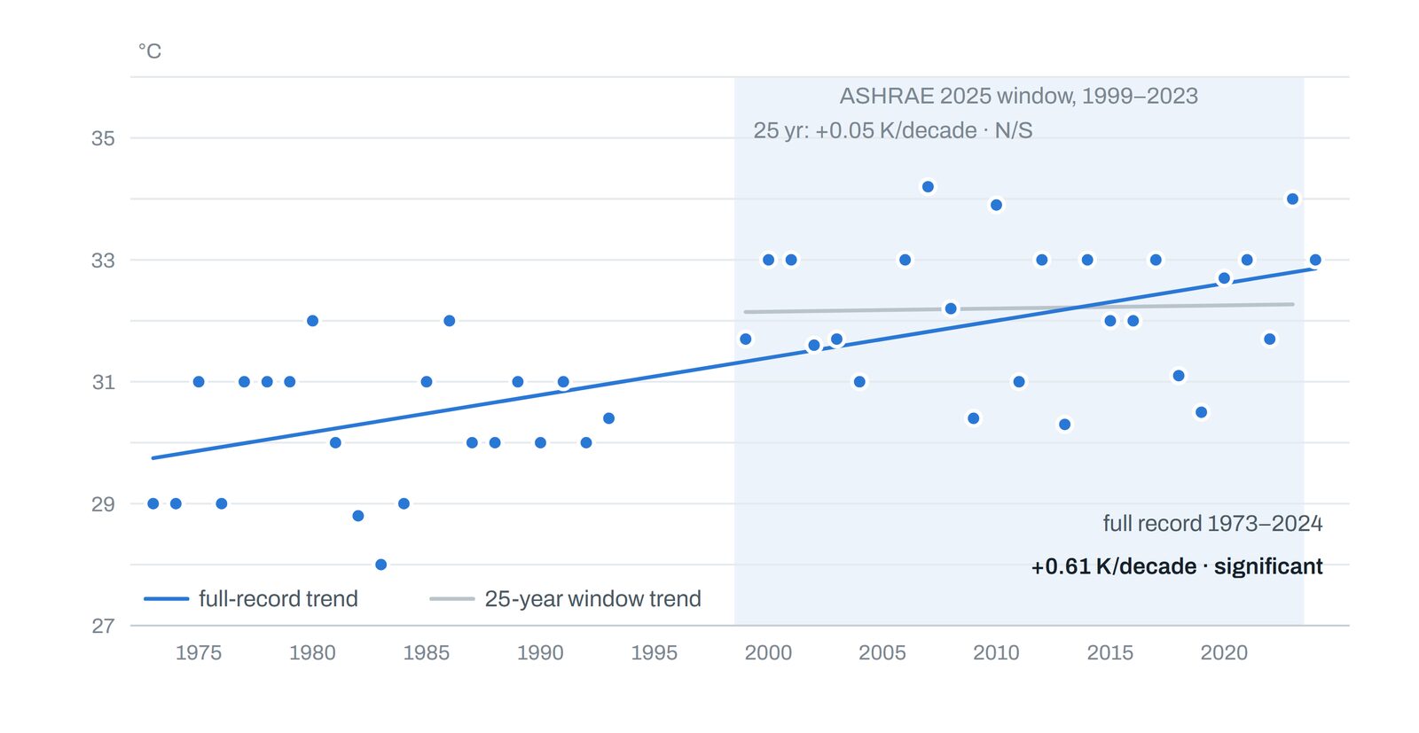
The slope of a yearly series is tested against its natural year-to-year scatter. With only 25 years of data, the smallest trend you can detect at 95 percent confidence stays around half a kelvin per decade at most stations. At the example station the threshold for the cooling design temperature is 0.66 K/decade in the 25-year window. When the full record is used (1973–2024, 46 usable years), the threshold drops to 0.21. The result is striking. Looking at the same series with the same method, the 25-year window returns a slope of +0.05 K/decade and the verdict “not significant”, while the full record returns +0.61 K/decade, clearly significant. Over a 30-year facility life, that rate corresponds to a shift of about +1.8 K.

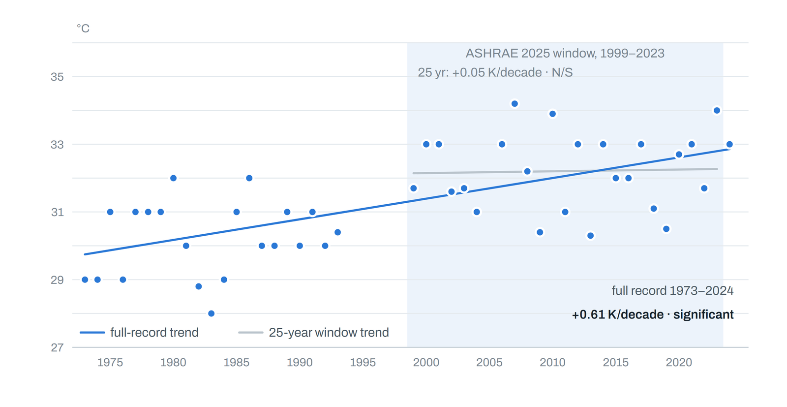
What this chart shows. Each blue dot is one year’s cooling design temperature. The grey line is the trend seen when only the last 25 years are used, and the blue line is the trend over the full record. In the short window the line is almost flat; once the record is extended, the warming becomes clearly visible.

Nor is this one station’s coincidence. We repeated the same computation in both windows at the 16 stations that have 30 or more usable years. In the 25-year window, the cooling design trend came out significant at just 1 station, exactly matching ASHRAE’s published count. In the full record it came out significant at 12 stations, all 12 positive, with a median of +0.37 K/decade.

A short window does not merely hide the trend; it can flip its sign. Seven of the 16 stations read negative in the 25-year window, while 15 of 16 are positive over the full record. In short, “N/S” does not mean the climate has stopped. It only means that 25 years is not enough to see the signal. Long records do need checks for station moves and instrument changes, but the direction and magnitude of the trend still read far more reliably from the full record.

3. Second limit: the station is not your site; the gap lives at night and the bill lands in PUE

An ASHRAE row describes conditions at a weather station, and it says so openly. The step nobody audits is the moment an engineer substitutes an airport 20 to 30 km away for the site. To measure what that step costs, we placed two records side by side at the example site. The national network’s station 8 km from the site was compared with ASHRAE’s station 26 km away over 23,851 matched hours covering three winters and three summers. The mean difference was −1.56 K; the site is colder than the station. The real information, however, sat in the daily pattern. At night the site was 2.0 to 2.5 K colder, while at midday the difference nearly vanished. That is the textbook signature of radiative cooling and cold-air pooling over open terrain. For a site inside the urban fabric the same mechanism works in reverse: the urban heat island makes the site warmer than a rural station suggests.

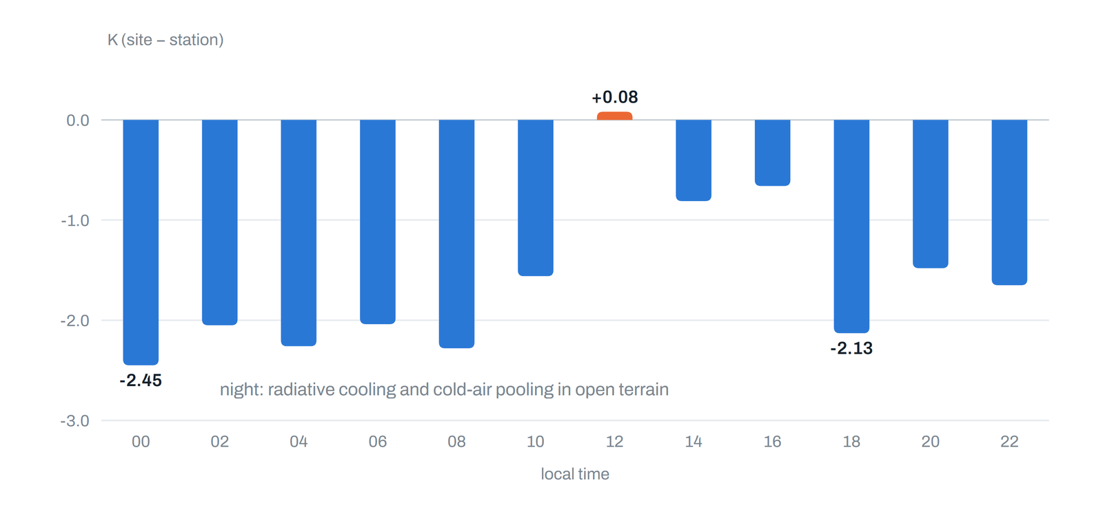
What this chart shows. The bars show how much the site differs from the station at each hour of the day. The gap is close to zero at the midday cooling peak and grows beyond 2 K at night. Station choice therefore affects winter design and free-cooling hours far more than the summer peak.

This asymmetry decides which design quantity absorbs the error. On the cooling side, the 0.4% dry-bulb value differs by only 0.3 K, and in the safe direction; a chiller sized to the station will not be undersized at the site. On the heating side, the 99.6% value is 2.1 K optimistic. Freeze protection, the glycol fraction, the dry cooler’s winter operating point and the humidification load all hang on that line. The free-cooling window is also 454 to 557 hours per year wider than the station suggests. One more thing is worth knowing: the station that best represents your site is usually not in the ASHRAE table at all, because national meteorological networks do not feed the international ISD archive. That is a matter of data plumbing, not data quality.

The correct transfer method follows from this. Take the absolute level from ASHRAE’s 25-year record and carry only the measured offset to the site. Write the tail offset as a band rather than a single number (here −2.3 ± 0.7 K). Reanalysis data such as ERA5 can serve as a bridge but not as a source; in this region it captured the cooling tail to within ±0.2 K yet showed a +2.3 K warm bias in the heating tail. What these lines mean depends on your role. For the investor they are megawatt-hours spread over a 25-year cash flow, for the designer they are freeze protection and glycol, and for the operator they are PUE.

4. Third limit: N50 is not a temperature but a promise, and the promise was made to the 2011 climate

N-year values are derived from a stationary Gumbel distribution fitted to the annual maxima of the last 25 years. The full meaning of “N50 = 41.0 °C” is therefore this: if the 1999–2023 climate lasted forever, this temperature would occur about once every 50 years. The centre of that window is 2011, and the climate is not stationary. According to IPCC AR6, a hot extreme that occurred once in 50 years in the pre-industrial climate already occurs 4.8 times per 50 years in a world warmed by +1 °C, roughly the world of the ASHRAE window, and 13.9 times at +2 °C. In other words, the “once in 50 years” label turns into roughly “once in 17 years” at +2 °C, and the threshold itself rises by about 1.5 K. “+2 °C” is not a date. Depending on the scenario it arrives between the 2040s and the 2050s, which is mid-life for a facility commissioned today.

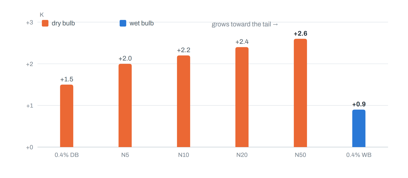
What this chart shows. The bars show that the climate delta is not a single number. The shift grows toward the tail of the distribution: +1.5 K at the 0.4% point but +2.6 K at N50. The blue bar shows that the wet bulb moves much more slowly, which is where evaporative and adiabatic designs earn their climate advantage.

Three subtleties matter in this calculation. First, global warming is not local warming. At the example location the mean temperature shifts by +1.35 K and the hot tail by +1.60 K, while the global mean warms by roughly +1 K over the same period; the local signal is about 1.5 times the global one. Second, the shift is not a single number. Because the spread of the annual maxima grows along with their mean, the delta increases toward the tail, and applying the 0.4% delta to every field understates N50 by about 1.1 K in this example. Third, dry bulb and wet bulb do not move together. In this continental dry climate the wet-bulb delta (+0.9 K) is about 60 percent of the dry-bulb one, which is why adiabatic-assisted designs age better as the climate shifts. In humid climates the ratio is different, and every site deserves its own arithmetic. Ready-made tools exist for this step (WeatherShift, CAHDC, ClimateData.ca, the CIBSE future weather files), and all of them add a model delta on top of an observed station value. As their own documents note, the uncertainty of that baseline and the station-to-site transfer remain out of scope. The first two terms stay on the engineer’s desk.

5. Capacity is decided in one hot afternoon; PUE is earned over a thousand cold nights

Two different questions need to be kept apart. The first is the capacity question: how many kilowatts of heat can I reject in the worst hour? The 0.4% percentile and the N-year extremes answer it, and the climate delta joins in through derating and through the outdoor temperature at which N+1 redundancy is evaluated. The second is the energy question: how many kilowatt-hours do the year’s 8,760 hours cost in total? Its answer is set not by the peak but by where the hours sit and by the machine’s efficiency at each temperature. At the example station, 52 percent of hours are below 12 °C and 72 percent below 18 °C, while hours at or above 30 °C total only 261 per year. In free-cooling mode the effective COP reaches the range of 10 to 20; in mechanical mode it falls to 3 to 6. Annual average COP, and with it PUE, is therefore earned in the cold and mild hours.

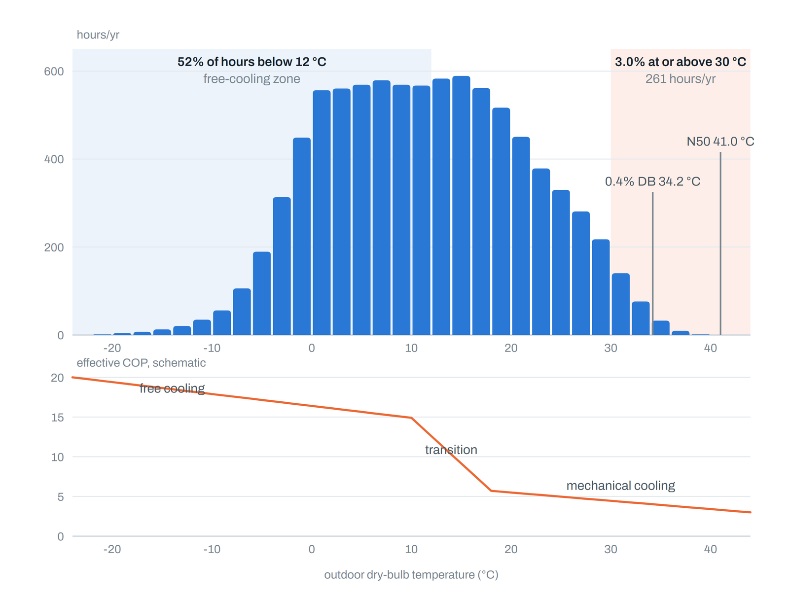
What this chart shows. The histogram shows where the hours of the year actually sit; the design points (34.2 °C and N50 41.0 °C) are far out in the nearly empty right-hand tail. The curve below sketches how efficiency is high in cold air and low in hot air. The energy bill is decided in the crowded cool part of the histogram, not at the peak.

Because the station-to-site gap grows largest at night and in winter, it hits the PUE model harder than the capacity sheet. A PUE model built on station data understates this site’s free-cooling window by 5 to 6 points, or 7 to 9 percent in relative terms. Given that PUE is now a metric reported to regulators in several markets, that gap is the business case itself. Winter matters in one more way: the heating design temperature is 2.1 K optimistic in this example, and the full record shows it warming significantly at 9 of the 16 stations. The free-cooling window will therefore narrow slowly over the facility’s life.

This picture also carries a message for cooling equipment manufacturers. The COP and capacity curves published for chillers, dry coolers and precision cooling units are usually measured at standard rating points. Yet the distribution above shows that annual energy is actually earned at part load and at low outdoor temperatures. Selection software becomes truly honest when it multiplies the full temperature-and-load-dependent efficiency curve by the site’s own hour distribution instead of quoting a single nominal COP. The changeover temperature to free cooling, the part-load efficiency and the winter operating limit are the most valuable parts of that curve. The economics are simple. Electricity is expensive, and you cannot always get as much of it as you want, wherever you want it. On a site with a limited grid connection, every point of PUE is power you cannot deliver to the IT load. A commitment made on an optimistic curve comes back later, either as an energy bill or as missing capacity. In short, capacity is decided in one hot afternoon, while energy is earned over thousands of cold nights, and the table measured those nights at the airport rather than at your site.

Not against ASHRAE, with ASHRAE

The conclusion of this article is not that ASHRAE is wrong; the data does not support that. The table is correctly computed, reproducible and honest about its own limits. On the cooling tail it represents the example site with an error of just 0.3 K, and on the safe side. What is wrong are the three silent assumptions that get attached to it: that 25 years reveals the trend, that the station represents the site, and that the climate is stationary. The situation resembles a flood map. The map is drawn correctly, but once a dam is built on the river, what needs updating is the label on the map. Updating that label is not the standard’s job. It is the job of the engineer who uses the standard, and it is exactly the work that investors, designers and operators should be asking to see on the table.

Related reading

• Data Center CFD & Thermal Analysis: White and grey space CFD through to time-dependent resilience scenarios.
• Meteorology & Climate Data: The observation and climate data layer behind design conditions.
• Energy Modelling: Annual energy and PUE assessment from 8,760-hour simulation.
• TSRS Climate Risk Reporting: Carrying physical climate risk into corporate reporting.
• UrClimate Score: Site-level climate projection and risk quantification.